Relational Database Management System: An Engineering Deep-Dive

Despite the meteoric rise of NoSQL, time-series, and vector databases in the last decade, the Relational Database Management System (RDBMS) remains the immutable backbone of global enterprise software. Whether it’s financial ledgers, inventory management, or user identity systems, the relational model’s promise of ACID (Atomicity, Consistency, Isolation, Durability) compliance and mathematical rigor is irreplaceable.
This article is not a high-level overview. We are going to deconstruct the RDBMS from the ground up—from the theoretical underpinnings of tuple calculus and storage architecture to the pragmatic realities of SQL optimization and schema normalization.
Unit 1: The Foundation – Architecture & The Relational Model
To engineer robust systems, one must understand what happens before a query is executed. An RDBMS is not merely a data bucket; it is a complex engine designed to bridge the gap between logical data representation and physical storage.
Purpose and View of Data
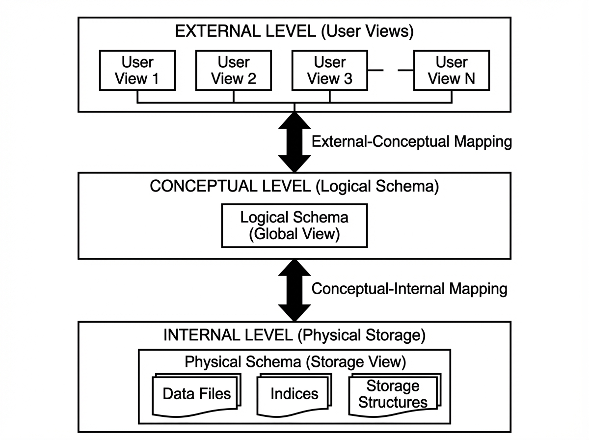
Legacy file processing systems suffered from data redundancy, isolation, and lack of atomicity. If a file transfer crashed halfway, data was corrupted. RDBMS solves this via Data Abstraction:
- Physical Level: How data is actually stored (block sizes, B-Trees, hashing).
- Logical Level: What data is stored and the relationships (Tables, Columns).
- View Level: Virtual tables (Views) that hide complexity or sensitive data from specific users.
Database Architecture
The architecture of a database determines its throughput and reliability. It is generally split into the Query Processor and the Storage Manager.
1. The Storage Manager
This is the interface between the low-level data stored in the OS file system and the application.
- Buffer Manager: Critical for performance. It manages caching data blocks in RAM to minimize expensive disk I/O. If your DB is slow, check your buffer pool hit ratio.
- File Manager: Manages allocation of space on disk structures.
- Transaction Manager: Ensures the system remains in a consistent state despite failures (Power loss, crashes).
2. The Query Processor
This is the “brain” of the operation.
- DDL Interpreter: Interprets schema definitions.
- DML Compiler: Translates SQL into an evaluation plan (relational algebra).
- Query Evaluation Engine: Executes the low-level instructions generated by the compiler.
The Relational Model
Proposed by E.F. Codd, the relational model is based on set theory.
- Relation (Table): A set of tuples.
- Tuple (Row): An ordered list of values.
- Attribute (Column): A named property of the relation.
- Domain: The set of permitted values for an attribute (e.g., Integer, Varchar).
Keys: The Guardians of Integrity
Keys are not just for indexing; they strictly define identity.
- Super Key: A set of one or more attributes that uniquely identify a tuple.
- Candidate Key: A minimal super key (no extraneous attributes).
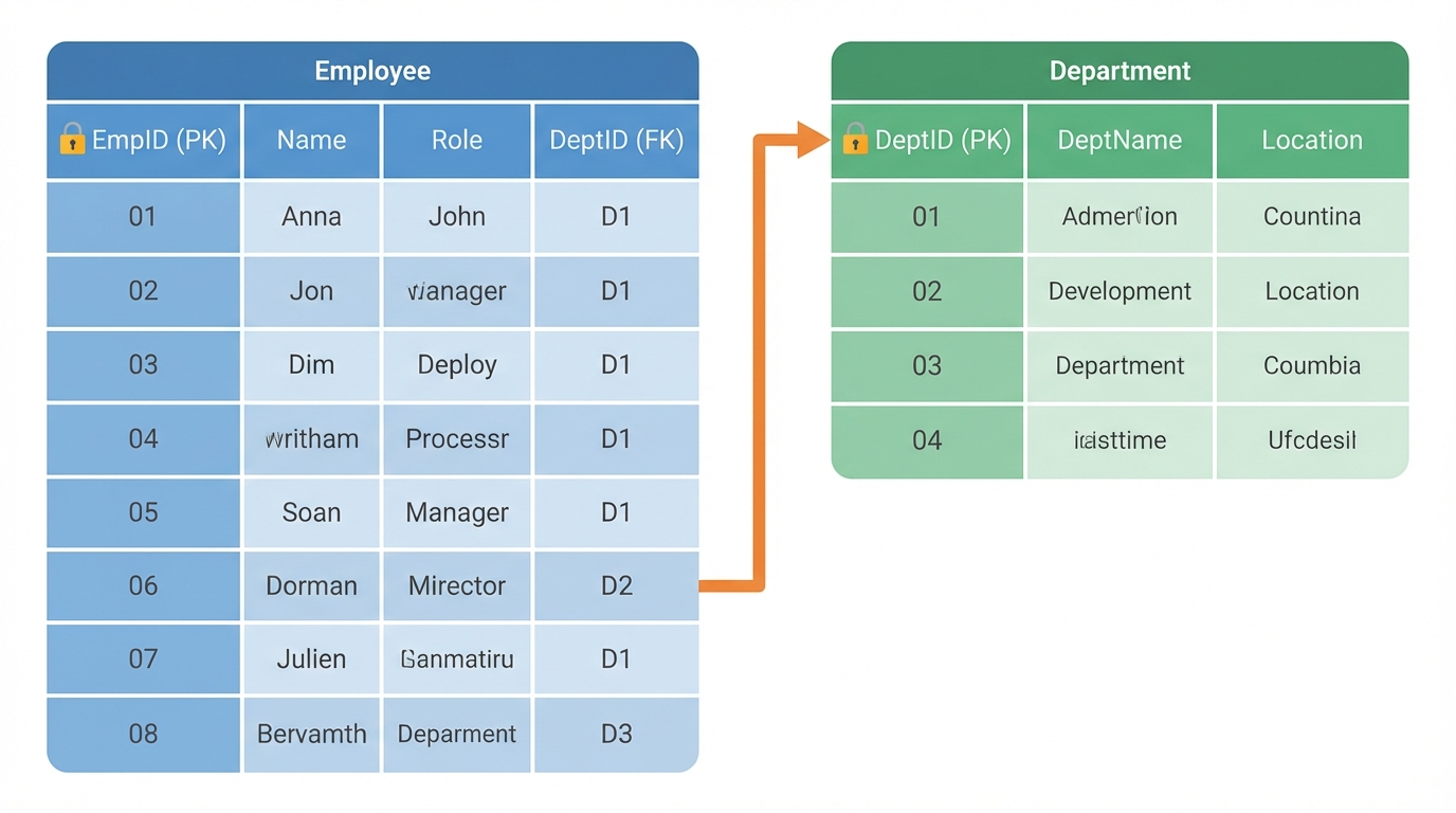
- Primary Key (PK): The candidate key chosen by the database designer as the principal means of identification.
- Foreign Key (FK): An attribute in one table that references the PK of another. This enforces Referential Integrity.
Scenario: If you have an Orders table referencing a Users table via user_id, the database engine (via FK constraints) physically prevents you from deleting a User who has active orders, preventing orphaned data.
Unit 2: Database Design & Normalization
A poorly designed schema is a technical debt that gathers interest at a compound rate. Database design is the process of converting real-world requirements into a mathematical model that minimizes redundancy.
Entity-Relationship (E-R) Model
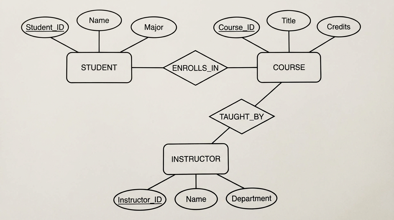
Before writing SQL, we model. The E-R model represents the world in terms of Entities (objects) and Relationships (associations).
Core Components
- Entity Sets: E.g.,
Employee. - Attributes: Properties like
SSN,Name.- Derived Attributes: Calculated from others (e.g.,
AgefromDOB). - Multivalued Attributes: E.g.,
Phone_Numbers.
- Derived Attributes: Calculated from others (e.g.,
- Relationships: The association between entities (e.g.,
Works_For).
Constraints & Cardinality
- One-to-One (1:1): CEO manages one Company.
- One-to-Many (1:N): Department employs many Employees.
- Many-to-Many (M:N): Students enroll in many Courses.
Design Issue - Reduction to Relational Schemas: When converting E-R to Tables:
- Strong Entity Sets become their own tables.
- Weak Entity Sets (depend on a strong entity for existence) include the strong entity’s PK as a Foreign Key.
- M:N Relationships require a Join Table (associative entity) containing the PKs of both participating entities.
Relational Database Design: Normalization
Normalization is the process of organizing data to reduce redundancy and improve data integrity. It relies heavily on Functional Dependencies (FDs).
Functional Dependency Theory
An FD is denoted as $X \rightarrow Y$. It means if two tuples agree on attribute $X$, they must agree on attribute $Y$.
- Axioms of Armstrong: Reflexivity, Augmentation, Transitivity. These allow us to infer new dependencies.
The Normal Forms
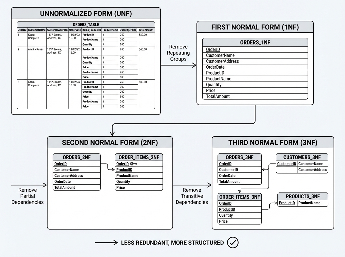
We decompose tables to eliminate anomalies (Update, Insert, Delete anomalies).
1. First Normal Form (1NF)
Rule: Attributes must be atomic. No repeating groups or arrays.
- Bad:
User(ID, Name, Phones)where Phones is “555-0101, 555-0102”. - Good: Move phones to a separate table
UserPhones(UserID, Phone).
2. Second Normal Form (2NF)
Rule: Must be in 1NF AND no Partial Dependencies.
- Context: Applies when the Primary Key is composite.
- Violation:
OrderItems(OrderID, ProductID, ProductName, Quantity). PK is(OrderID, ProductID).ProductNamedepends only onProductID, not the whole key. - Fix: Split into
Products(ProductID, ProductName)andOrderItems(OrderID, ProductID, Quantity).
3. Third Normal Form (3NF)
Rule: Must be in 2NF AND no Transitive Dependencies.
- Violation:
Employee(ID, ZipCode, City).ID -> ZipCode, butZipCode -> City. - Fix:
Employee(ID, ZipCode)andLocations(ZipCode, City).
4. BCNF (Boyce-Codd Normal Form)
A stricter version of 3NF. For every FD $X \rightarrow Y$, $X$ must be a super key. This handles edge cases where a prime attribute depends on a non-prime attribute.
Decomposition Algorithm: When decomposing tables, two properties must be preserved:
- Lossless Join: Can we join the tables back to get the original data without creating spurious rows?
- Dependency Preservation: Can we enforce constraints without joining tables?
Unit 3: SQL Basics – Definition & Control
SQL (Structured Query Language) is the implementation of the relational model. It is declarative: you tell the DB what you want, not how to get it.
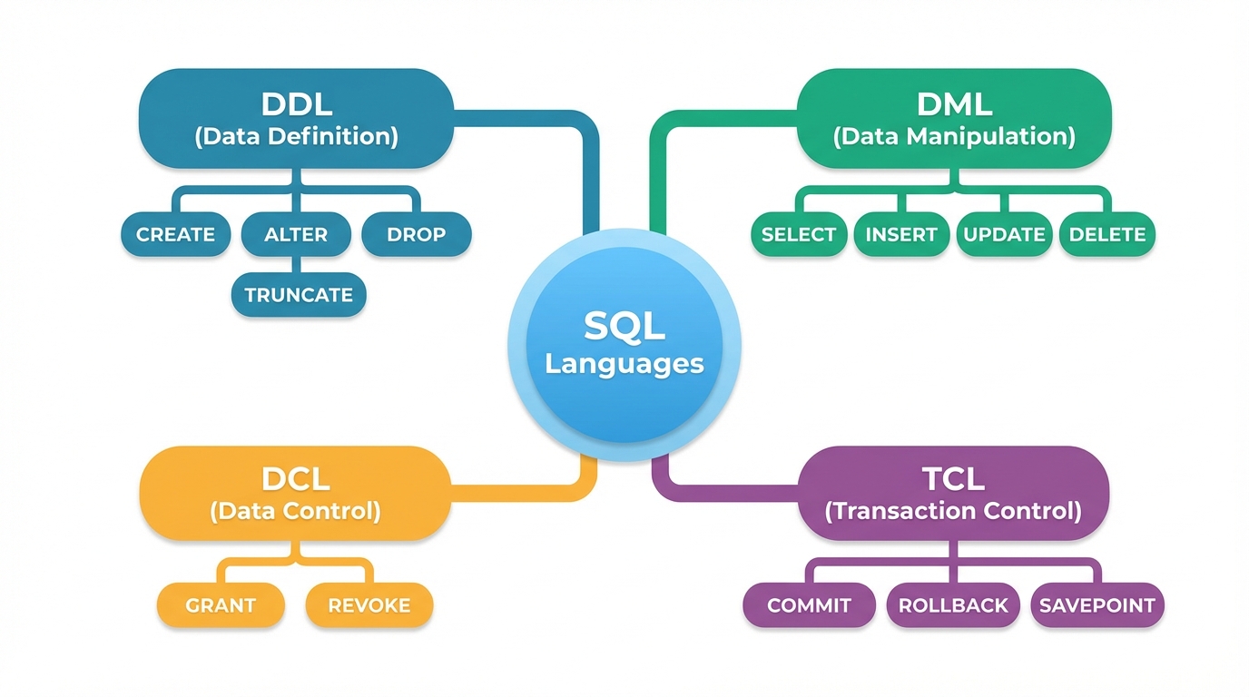
Data Definition Language (DDL)
DDL defines the structure. In a production environment, DDL is dangerous. Locking a table to add a column can bring down a high-traffic service.
Creating Tables with Constraints
CREATE TABLE Employees (
    emp_id INT PRIMARY KEY,
    email VARCHAR(255) UNIQUE NOT NULL,
    salary DECIMAL(10, 2) CHECK (salary > 0),
    dept_id INT,
    hire_date DATE DEFAULT CURRENT_DATE,
    CONSTRAINT fk_dept
        FOREIGN KEY (dept_id)
        REFERENCES Departments(dept_id)
        ON DELETE SET NULL
);
- Constraint Naming: Always name your constraints (
fk_dept). It makes debugging error logs significantly easier. - Types:
INT,VARCHAR,DECIMAL(for money—never use FLOAT),DATE.
Altering and Dropping
-- Adding a column
ALTER TABLE Employees ADD COLUMN phone_number VARCHAR(20);

-- Renaming (Database specific, standard SQL uses RENAME TO)
ALTER TABLE Employees RENAME TO Staff;

-- Truncate vs Delete
TRUNCATE TABLE Staff; -- Fast, resets High Water Mark, no undo (DDL)
DELETE FROM Staff;    -- Slower, logs every row, transactional (DML)
DCL (Data Control Language)
Security is paramount.
GRANT SELECT, INSERT ON Employees TO app_user;
REVOKE DELETE ON Employees FROM app_user;
Error Codes & Spooling
- Spooling: In CLI tools (like SQL*Plus), spooling directs query output to a file. Useful for generating CSV reports via cron jobs.
- Error Codes: Applications should trap SQLSTATE codes. For example, a duplicate key violation usually returns specific codes (e.g., 23505 in Postgres) allowing the app to fail gracefully.
Unit 4: Data Management, Retrieval & Functions
This is where the rubber meets the road. Writing efficient DML (Data Manipulation Language) is the primary skill of a backend engineer.
DML: Managing Data
The INSERT, UPDATE, and DELETE statements are straightforward but powerful.
-- Multi-row insert
INSERT INTO Products (name, price) VALUES
('Widget A', 10.00),
('Widget B', 15.50);

-- Update with logic
UPDATE Employees
SET salary = salary * 1.05
WHERE performance_rating > 4;

-- Substitution Variables (Tool specific, e.g., SQL*Plus)
-- DEFINE department_id = 10;
-- SELECT * FROM Employees WHERE dept_id = &department_id;
Advanced Retrieval: The SELECT Anatomy
The execution order of a SQL query is different from the writing order:
- FROM / JOIN (Gather data)
- WHERE (Filter rows)
- GROUP BY (Aggregate)
- HAVING (Filter groups)
- SELECT (Return columns)
- ORDER BY (Sort)
Conditional Logic: CASE
The CASE statement allows for if-then logic directly in the projection.
SELECT
    name,
    salary,
    CASE
        WHEN salary < 50000 THEN 'Junior'
        WHEN salary BETWEEN 50000 AND 100000 THEN 'Mid'
        ELSE 'Senior'
    END as seniority_level
FROM Employees;
Multiple Tables: Joins
Joins are the physical realization of the Cartesian product filtered by a predicate.
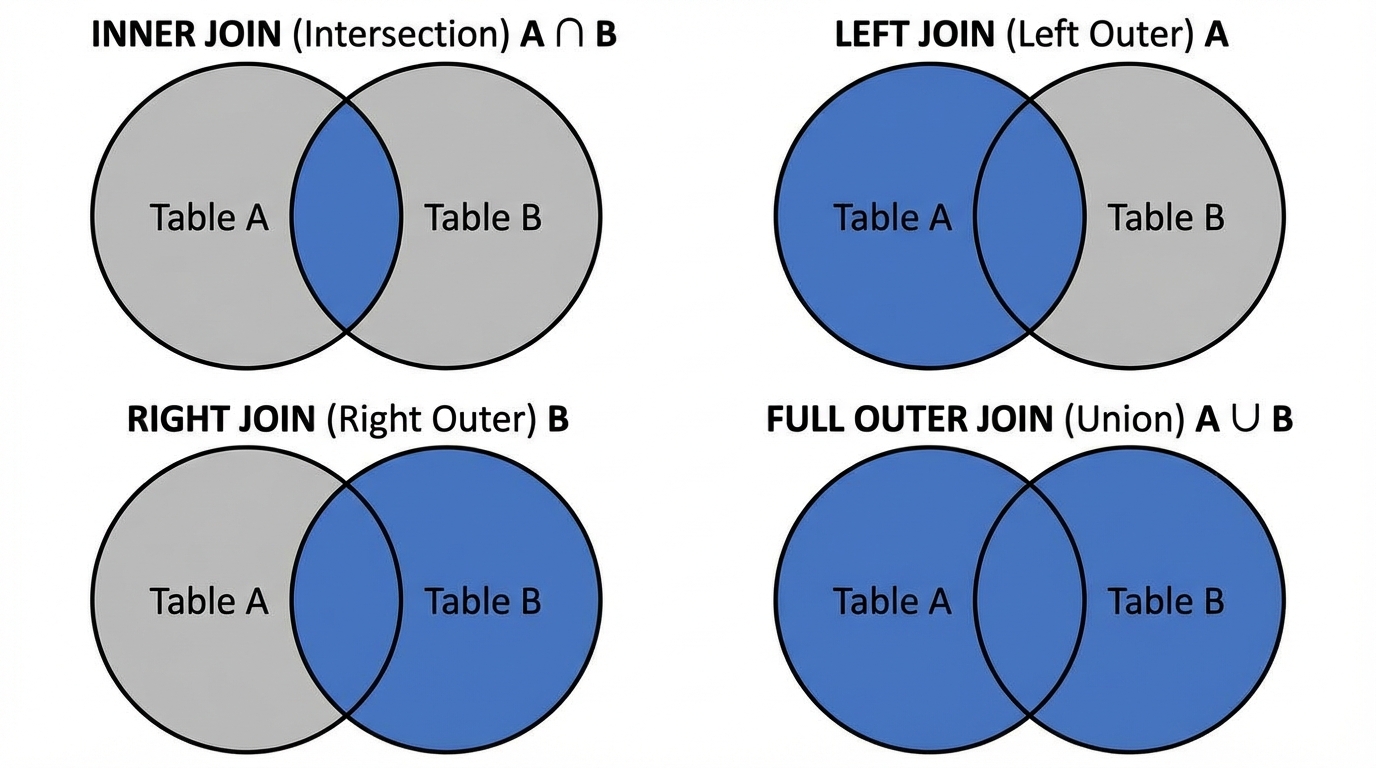
- Inner Join: Returns rows when there is a match in both tables.
- Left (Outer) Join: All rows from the left table, and matched rows from the right table (NULL if no match).
- Right (Outer) Join: Inverse of Left Join.
- Full Join: All rows from both tables.
- Self Join: Joining a table to itself (e.g., Employee hierarchy where Manager is also an Employee).
SELECT
    e.name as Employee,
    m.name as Manager
FROM Employees e
LEFT JOIN Employees m ON e.manager_id = m.emp_id;
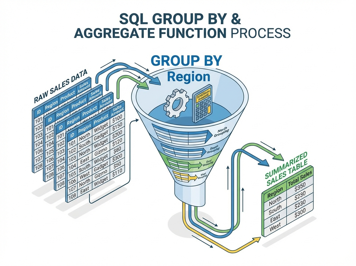
Functions and Grouping
Aggregation reduces multiple rows into a single summary value.
Built-in Functions
- Numeric:
ROUND(),TRUNC(),MOD(). - String:
UPPER(),SUBSTR(),CONCAT(). - Date:
ADD_MONTHS(),EXTRACT(YEAR FROM date).
Grouping and HAVING
The HAVING clause is essential because the WHERE clause cannot filter on aggregate functions (because WHERE runs before aggregation).
Scenario: Find departments where the average salary is greater than $80,000.
SELECT
    dept_id,
    AVG(salary) as avg_sal
FROM Employees
WHERE status = 'Active'  -- Filter raw rows first
GROUP BY dept_id         -- Aggregate
HAVING AVG(salary) > 80000; -- Filter the aggregates
Set Operations
These combine the results of two separate queries.
- UNION: Combines results, removes duplicates.
- UNION ALL: Combines results, keeps duplicates (Faster).
- INTERSECT: Returns only rows present in both sets.
- MINUS / EXCEPT: Returns rows in the first set but not the second.
Conclusion
The Relational Database Management System is a triumph of computer science, blending rigid mathematical theory with practical software engineering. From the low-level Storage Manager optimizing disk access to the high-level SQL logic handling complex joins and aggregations, the RDBMS is designed for data integrity and reliability.
As you design systems, remember:
- Normalize to ensure consistency, but be willing to Denormalize judiciously for read performance.
- Constraints are your friends; let the database enforce the rules, not just the application code.
- Understand the Execution Order of SQL to write performant queries.
Mastering these units provides the capability to handle not just a few thousand records, but to architect systems that scale to terabytes of mission-critical data.